Sample Super Store Analysis Using Python & Pandas (Part 01)

1. Introduction

This tutorial is intended to give some quick, fundamental and brief overview on how to explore a dataset, which in this case is the Sample SuperStore. And to my best knowledge, it's coming from a fictional e-commerce or online marketplace company's annual sales figures. But the bottom line, the dataset would provide you with sufficient information on how you may work with an actual real life data. Among other things, this dataset consists of the following data types that may showcase the actual capabilities of what Pandas capable of delivering.

• Timestamp or the timeseries datatypes.
• Both Category and SubCategory elements datatypes.
• Numerical datatypes, so we may perform couple of numerical analysis.
• From the previous point, we sure can perform another features generation on this dataset.

And with that being said, let's try to explore further the dataset, with the various built-in functionalities in the Panda's library for Python have to offer, while utilizing the Jupyter Notebook as the main IDE of choice. And please don't forget to download the CSV file used on this project, you can download it from my GitHub account found here.

2. Installation

First and foremost, this data exploration would assume you, to have one proper and working installation of the Python programming language. Secondly you have the Jupyter Notebook and the Pandas library installed on your workstation, which we will use throughout the course of this data exploration.

While the installation part for each of the mentioned pieces of software mentioned go beyond the scope of this tutorial, I would suggest that you head over to the official sites, and there you may discover further steps on how to download, install and setup the required programming language and libraries according to your operating systems. Once that you have settled with the whole installation and configuration issues, you may come back again to this page and follow along the instructions.

• Python Official Website.
• Panda's Official Website.
• Jupyter Official Website.

3. Importing Library

Next, we need to load the Panda libraries onto our Jupyter Notebook environment. This way, it would tell Python, through the means available at Jupyter Notebook, to boot-up so we could utilize its built-ins functionalities available. Here's a snippet on how to do load your Pandas to Jupyter Notebook environement:

# Importing packages
import pandas as pd

Now, that we have settled our first challenge, let's move further to read the datasets coming from a CSV file.

4. Reading Dataset

The following code would imply these instructions

• _df_orders_ = is the name of the variable, that will be using throughout the example of this tutorial.
• pd = stands for Panda, it's the convention the community is using.
• _.read_csv_ = is a method within to read the CSV file.
• _index_col_ ='Order ID'

# Let's try to read from the superstore.csv
df_orders = pd.read_csv('data/superstore.csv')

If you notice form the above code, it's implying that we need to put our superstore.csv dataset on a directory called data. So once that you download the dataset, create a folder named data and put your superstore.csv file there on that particular directory or folder.

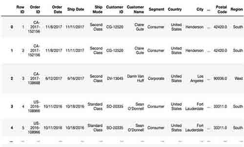
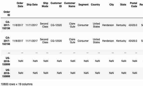
This is the default view of a dataset in Jupyter Notebook

By default, Panda's built-in functionality, only showing 20 columns and 10 rows for each dataset, every time time you try to display them in the view. If you notice from the tabular data above, the dataset get truncated with triple dots sign '...' both for the rows and the columns. And since this dataset has 10800 rows with 21 columns, it'll only show the first 10 records for the row, with only 20 columns to the right instead of 21. As a side note, you can scroll the dataset both to the right and to the bottom, that way you can see the actual dataset content.

5. Dropping The "Row ID"

The "Row ID" column is not really that informative, I think it would be safe enough for us to simply just delete them. That way, it would give us much more clarity over our dataset.

• _df_orders_ = is the name of the variable, that will be using throughout the example of this tutorial.
• .drop = the method being used to drop column.
• inplace=True = we used them to keep the changes onward.

df_orders.drop("Row ID", axis=1, inplace=True)

# Let's call the previously defined data variable, the 'df_orders'
df_orders

The first column has been changed from 'ROW ID' to 'Order ID'

As you can see from the above table, we don't have the 'ROW ID' no longer in place and instead, it's being replaced by the 'Order ID'.

6. Change "The Index" Column

By each time you're using pd.read_csv('somedata.csv'), that would yield the dataset's actual rows and columns, and we certainly have quite an extensive records of data, as being displayed from the previous function.

As you may notice, the first column isn't the actual "Row ID" column, rather it's the default built-in feature Panda's bringing into the dataset. Let's try to change that into something much more useful. Now, let's revisit our previous Panda's function, but this time we add another parameter, the _"index_col"_ to be exact.

Since that we wish to redo them again over a clean dataset, let's just call them again one more time with the
'df_orders = pd.read_csv('data/superstore.csv', index_col='Order ID')' function.

Let's continue with the 'df_orders' variable again. So don't be surprise if you see the 'Row ID' column reappearing in the dataset since that would illustrate best our objective, but this time the 'index column' values have changed from the value coming from the 'Order ID' column instead.

# Let's try to read again from the superstore.csv
df_orders = pd.read_csv('data/superstore.csv', index_col='Order ID')
# added the index_col='Order ID', parameter.

# Let's call the previously defined data variable, the 'df_orders'

df_orders

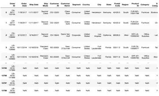
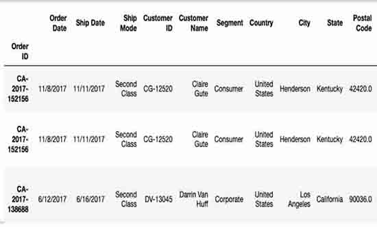
The Index column has been changed, from default builtin, to 'Order ID' column.

Once that we tried to add the additional parameter, as you may notice, the first column have changed to 'Order ID' column, rather then the previous Panda's built-in index column, and the other thing was, the fine print below each table now have changed, from 21 columns, to only 20 columns instead.

7. Drop the Row ID & Change The Index

On to our another objective, what if we wish to combine both of the features, with dropping the 'Row ID' and to change the 'Index' columns at the same time, so that we could get even leaner dataset to work with. With that kind of objective, we might need to combine both of the syntax to achive our objective.

df_orders.drop("Row ID", axis=1, inplace=True, index_col='Order ID')

• .drop() = this method to drop a column from the dataset.
• axis=1 = is the attribution value, on the dataset.
• inplace=True = we used them to keep our changes onward.
• index_col = make the defined column value, as our newly active index column instead.

df_orders = pd.read_csv('data/superstore.csv', index_col='Order ID')
df_orders.drop("Row ID", axis=1, inplace=True)

# Let's call the dataset again.
df_orders

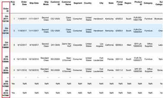
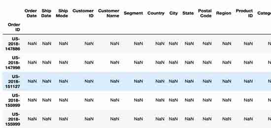
The Index column has been changed, from default builtin, to 'Order ID' column.

Now, as you may see, from the below printed information, we only have 19 columns remaining left, coming from the initial 21 columns previously being shown. Now you may ask, "But how come it's down to 19 columns, while we recall we only dropped 1 column?". The answer to that is due to the 'index_col' method, whereas we define the 'Order ID' to settle as the Index of the dataset. Pandas doesn't count that to a column, rather just another indexing attribution in the dataset.

8. Default Number Rows & Columns

Let's try to set the maximum column and row to display, since by default the pandas library would display 10 records of rows in total for a single dataset. The first 5 would coming from the top records, and the remaining would be coming from the last 5 records as a whole.

But that's a little too much of information anyone could digest in a short glimpse, why don't we just minimize them down to 5 records instead. The same thing with the columns view, whereas Pandas would display you 20 columns, but since our current dataset only have 19 of them, then that should be fine.

• _pd.set_option('display.max_columns', 20)_ = setting the default column's view.
• _pd.set_option('display.max_rows', 5)_ = setting the default row's view.

# Let's try to read from the superstore.csv
pd.set_option('display.max_columns', 20)
pd.set_option('display.max_rows', 5)

# Let's try to give it a go with the new setting.
df_orders

Changing the default view in Pandas (illustration got truncated).

9. The Dataset First 5 Rows

Here's another Pandas built-in method that may come handy. When you fell like taking a quick peek of the first 5 recrods from the top, the following code would deliver you those ouputs.

• _df_orders_ = is the name of the variable, that will be using throughout the example of this tutorial.
• .head() = is the method to display the first five records of data coming from the dataset.

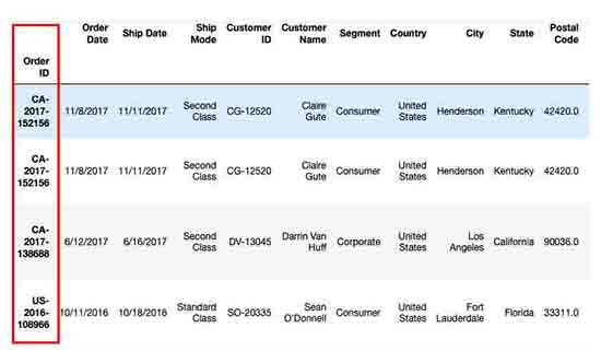
df_orders.head()

Viewing the first 5 rows of a dataset (illustration got truncated).

10. The Dataset Last 5 Rows

Much like the above previous syntax, the similar can be apply to the bottom 5 records coming from your dataset. And you guess it right, the syntax would be .tail() and that would give you the last 5 records from the dataset.

• df_orders = is the name of the variable, that will be using throughout the example of this tutorial.
• .tail() = is the method to display the last five records of data coming from the dataset.

Viewing the last 5 rows of a dataset (illustration got truncated).

11. The Dataset Structure

Now that you have one finer understanding on the previous aspect of importing library, loading the dataset and manipulate the views of the rows and the columns, let's now move on to the Dataset structure aspect. Whereas it's also an important area, before continuing the journey of exploring the dataset further.

The dataset you get from the wild, might not always have the proper structure and data types you need. And before you could do further analysis and manipulation, let's make sure that both the structure and data types have been taken care of properly.

12. Rows & Columns

Following are both the built-in method to achive our next objective, as we go more deeper over the analysis part of the dataset. Let's try to understand further of what how many rows and columns are there, we know this information from the previous part, but lucky for us, Pandas also provide us with a method di display the information in hand.

• _df_orders_ = is the name of the variable, that will be using throughout the example of this tutorial.
• .shape() = is the method to display the number of rows and column.

df_orders.shape

(10800, 19)

Aside from the fact, there are various other ways for us to know how many Rows and Columns available in your dataset, Pandas also has a builtin method to dispay those information. So now we understand that the dataset has the following total of information records.

• 10800 coloumns
• 19 coloumns

13. Dataset Columns

Imagine that you're working with a large dataset, and by large, not just merely on the amounts of rows that it'd produce. But also on the amount of columns spreaded from left to right. Good thing we're only working a 19 columns (from previously 21 columns in our dataset), now wouldn't it be nice to have a method to display all the columns available in our dataset? Well the good news is, Pandas shipped with a builtin method just to achive that.

• _df_orders_ = is the name of the variable, that will be using throughout the example of this tutorial.
• .columns = is the method to display all the columns available in the dataset.
• .dtypes() = is the method to display the data types from the dataset available.

# Let's print the columns (features) names.
df_orders.columns

Index(['Order Date', 'Ship Date', 'Ship Mode', 'Customer ID', 'Customer Name',
       'Segment', 'Country', 'City', 'State', 'Postal Code', 'Region',
       'Product ID', 'Category', 'Sub-Category', 'Product Name', 'Sales',
       'Quantity', 'Discount', 'Profit'],
      dtype='object')

14. Renaming Columns

Now it's just my way of doing things over the EDA aspect, is trying to eliminate any white spaces in between the columns name. It gets better and you may benefit alot from performing this method, and as we move on to something that's much more complicated within the data exploration, we'll benefit on the clarity aspect, too.

• _df_orders_ = is the name of the variable, that will be using throughout the example of this tutorial.
• .columns = is the method to rename the column names.

# Let's try to rename the column.
df_orders.columns = ['OrderDate', 'ShipDate', 'ShipMode', 'CustomerID', 'CustomerName', 'Segment' , 'Country', 'City', 'State', 'PostalCode', 'Region', 'ProductID', 'Category', 'SubCategory', 'ProductName' , 'Sales', 'Quantity', 'Discount', 'Profit']

df_orders

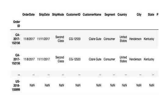
The columns after being renamed. (illustration got truncated).

15. Columns Data Type

Many times before you wish to explore further your columns in a dataset with some operation, you may need to make sure it's the correct data type that you're working with. For example, you wouldn't be able to do a division operation over a Timestamp data format, or multiply a String with with another string for that matter.

• _df_orders_ = is the name of the variable, that will be using throughout the example of this tutorial.
• .columns = is the method to display all the columns available in the dataset.
• .dtypes() = is the method to display the data types from the dataset available.

# Let's print the columns data types.
df_orders.info()

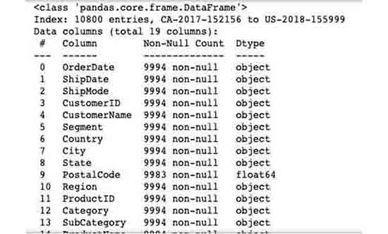
Viewing the data types of the dataset (illustration got truncated).

16. Incorrect Columns Data Type

As we can see from the above snippets, we have noticed there are couple of columns data types that were set incorrectly. For instance, the OrderDate data type was set to object data type instead of datetime, or the PostalCode was set to float data type, though you wouldn't do any calculation on top of it. Somewhere down the line with that kind of flaws, will lead us to even bigger problem if we don't try to fix them now. Let's try to patch those data types with the following methods.

• _df_orders_ = is the name of the variable, that will be using throughout the example of this tutorial.
• .astype = is the method to change the coloumns data type in the dataset.

# Let's try to change the datatypes of the following column in the dataset.
df_orders['OrderDate'] = df_orders['OrderDate'].astype('datetime64[ns]')
df_orders['ShipDate'] = df_orders['ShipDate'].astype('datetime64[ns]')
df_orders['PostalCode'] = df_orders['PostalCode'].astype('object')

And now let's try to recheck them again, to see if the codes have worked as intended.

# Let's print the columns data types.
df_orders.info()

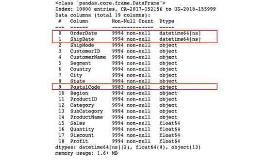
We've now changed the data types.

17. Dataset Statistic Figures

If you're more into the statistician type, perhaps you may be also interested by the following methods to generate the figures with only a single line of .describe Pandas method.

• _df_orders_ = is the name of the variable, that will be using throughout the example of this tutorial.
• .describe = is the method to pull out some statistics figures from the dataset.
• Short note, the .describe method would only work for numerical coloumn, and not categorical.
• While for the (include='all'), would work on both numerical & categorical values.

# Describing statistical information on the dataset
df_orders.describe()

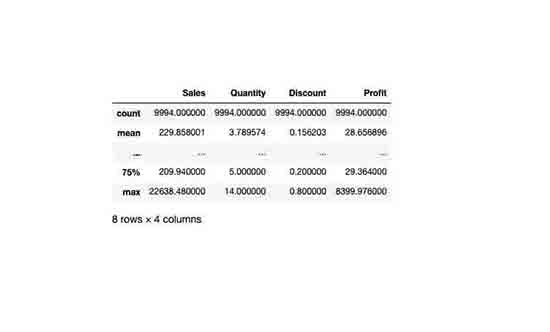
Decent Statistic Facts on The Dataset.

# Describing more statistical information on the dataset
df_orders.describe(include='all')

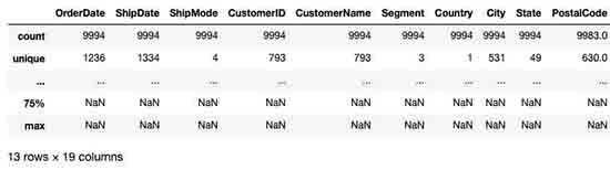
Decent Statistic Facts on The Dataset.

18. Statistic Figures

The following code would imply these instructions

• _df_orders_ = is the name of the variable, that will be using throughout the example of this tutorial.
• .count = is the count value to a specific column.
• .mean = is the std value to a specific column.
• .min = is the min value to a specific column.

df_orders["Sales"].count()

Would give you the value of "9994".

df_orders["Sales"].mean()

Would give you the value of "229.8580008304938".

df_orders["Sales"].std()

Would give you the value of "623.2451005086818".

df_orders["Sales"].min()

Would give you the value of "0.444".

19. Exporting Dataset

Once that we've satisfied with our results, it's time to export them. So let's export them a new CSV dataset, so we could work with them on the next notebook tutorial.

• _df_orders_ = is the name of the variable, that will be using throughout the example of this tutorial.
• _.to_csv_ = = is the export method to a CSV dataset.
• index = False = we need to definet this index value set to False, since we don't want the index column.

df_orders.to_csv('data/df_orders_exported.csv', index =False)

Now go ahead and check your current working directory. you may find your df_orders_exported.csv there.

20. Bonus Stage

Now that we've come a long way of exploring our superstore.csv dataset, it's time to dive a little bit deeper of what, both Python and Pandas capable of delivering. Let's try to create a custom class in Python by leveraging our builtin Pandas method available in the library.

# Let's create a class named `display_all`, by which later we call on the next command.
def display_all
(df_orders):
with pd.option_context("display.max_rows", 1000, "display.max_columns", 1000):
        display(df_orders)

What it does basically, it creates a class named display_all and called the df_orders variable that we've defined earlier at the top of this jupyter notebook tutorial. Next, we call the pd.option_context method that would provide us with the display.max_rows and the dispplay.max_columns attributions. And lastly we combine them all in the display() method by the end of the class.

Now that we've combine them all together, let's put them into action, and see what it delivers back to us this time.

display_all(df_orders.head(10).T)

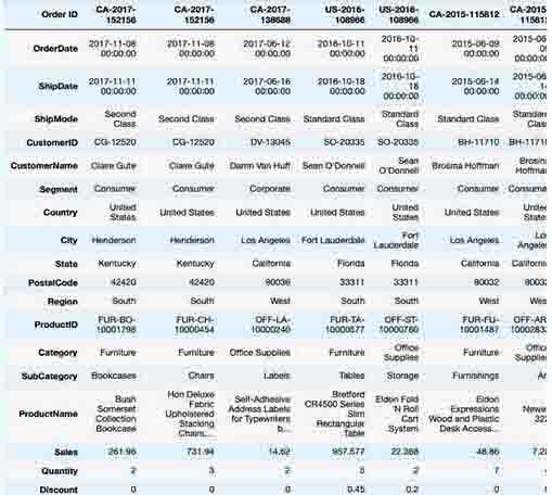
Now the dataset getting transposed in the view.

display_all(df_orders.describe(include='all').T)

Since we've defined the display_all from the previous class, we can now use it to explore further and combine them with different methods available in Pandas, much like the .describe attribute.

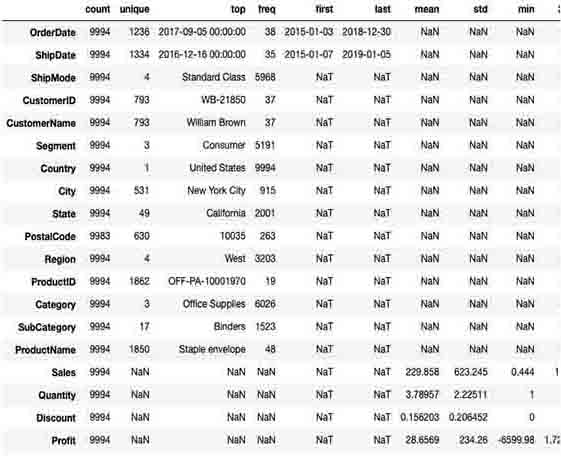
Now the Statistic from the dataset getting transposed in the view.

You've made it this far, congratulations on achieving your first essential data-scienctist project. But there's more, if you wish to explore further or perhaps want to experiment, fork this Jupyter Notebook else even copy them to your working directory. I made everthing available on my GitHub repository. Got any questions? Fell free to ask them down below in the comment section, I'll try to get back to any inquiries as soon as I could. Hope you enjoy this tutorial, and thank you for reading them.

---